HW 03: Non-linear and GLS models

FW8051 Statistics for Ecologists

Polynomials versus splines

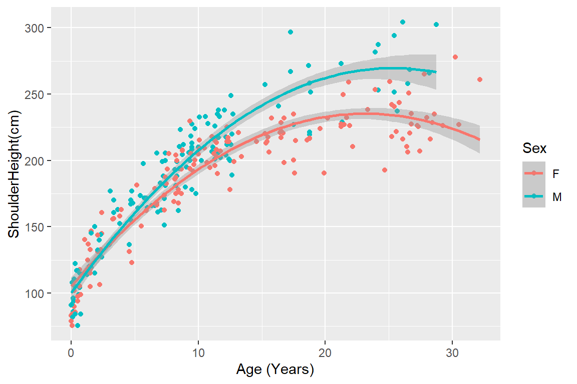
Both are acceptable and can capture the non-linear relationship between height and age, but a quandratic will eventually “bend” (up or down) in both directions.

ggplot(ElephantsMF, aes(x=Age,y= Height,color=Sex)) + 
  geom_point() + 
  geom_smooth(method="lm", formula= y~ poly(x, 2), se=TRUE) + 
  xlab("Age (Years)") +ylab("ShoulderHeight(cm)")

ggplot(ElephantsMF, aes(x=Age,y= Height,color=Sex)) + 
  geom_point() + 
  geom_smooth(method="lm", formula= y~ ns(x, 3), se=TRUE) +
  xlab("Age (Years)") +ylab("ShoulderHeight(cm)")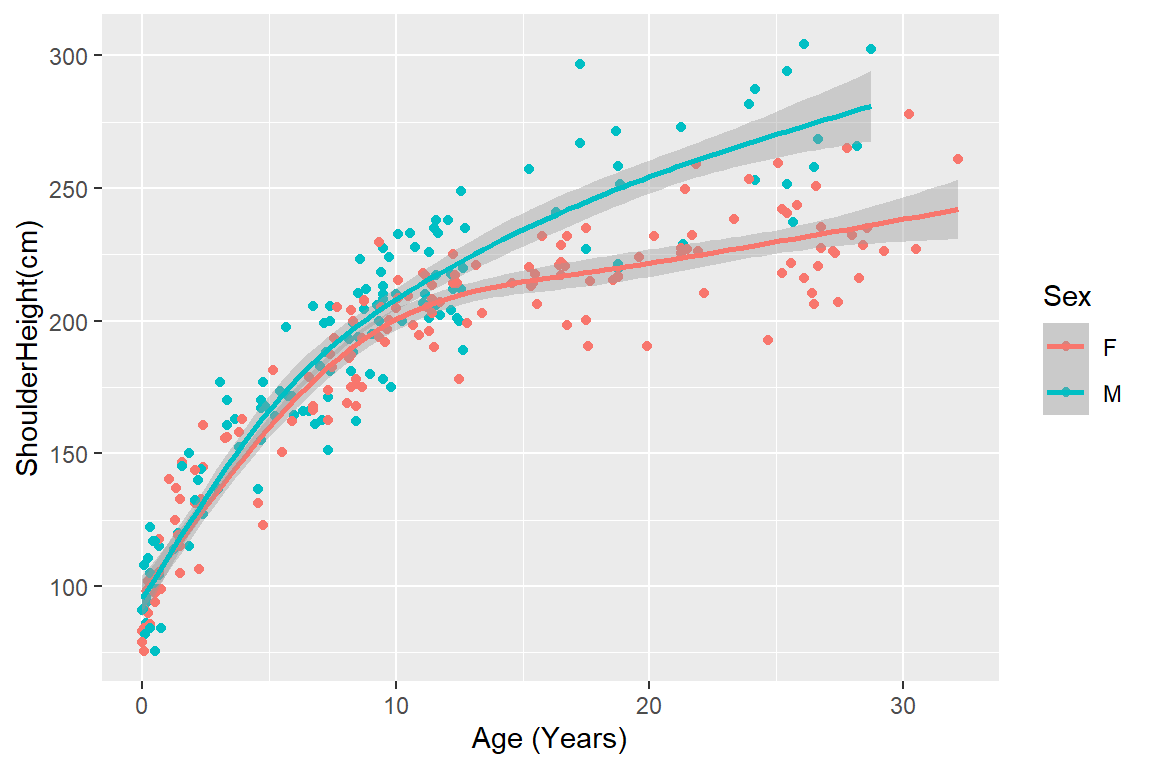

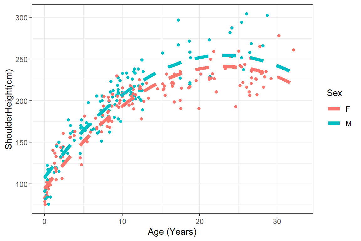
Plots

Mapping color to Sex results in an interactive model being plotted:

lm.ele <- lm(Height ~ Sex*poly(Age, 2), data = ElephantsMF)

That is not this model:

lm.ele <- lm(Height ~ Sex + poly(Age, 2), data = ElephantsMF)

ggplot(ElephantsMF, aes(x=Age,y= Height,color=Sex)) + 
  geom_point() + 
  geom_smooth(method="lm", formula= y~ poly(x, 2), se=TRUE) + 
  xlab("Age (Years)") +ylab("ShoulderHeight(cm)")

newdata <- data.frame(expand.grid(Sex = c("M", "F"), 
                                  Age = seq(0, 33, by = 1)))
newdata$phat <- predict(lm.ele, newdata =newdata)
ggplot(ElephantsMF, aes(x=Age,y= Height,color=Sex)) + 
  geom_point() + 
  geom_line(data = newdata, aes(Age, phat, col = Sex), lty =2, lwd =2)+
  xlab("Age (Years)") +ylab("ShoulderHeight(cm)") +
  theme_bw()

Number of knots (or df): Cubic regression splines

Could in principle compare models (e.g., using AIC) that have varying numbers of knots, or different knot locations

• Danger of overfitting, and difficult to account for model-selection uncertainty

Choose a small number of knots (df), based on how much data you have and how complex you expect the relationship to be a priori

• 2 or 3 internal knots are usually sufficient for small data sets
• Keele (2008), cited in Zuur et al, recommend 3 knots if \(n < 30\) and 5 knots if \(n > 100\)

Linear regression versus GLS models

Linear regression:

\[TF_i \sim N(\mu_i, \sigma^2)\] \[\mu_i = \beta_0 + \beta_1DBH_i\]

Minimizes \(\sum_i (TF_i - \beta_0 + \beta_1DBH_i)^2\)

GLS varPower model:

\[TF_i \sim N(\mu_i, \sigma_i^2)\] \[\mu_i = \beta_0 + \beta_1DBH_i\] \[\sigma_i = \sigma^2|DBH_i|^{2\delta}\]

Minimizes: \(\sum_i \frac{(Y - \beta_0 + \beta_1DBH_i)^2}{\sigma^2|DBH_i|^{2\delta}}\)

Estimates (SE) from the two models.

	linear model	varPower
(Intercept)	0.196 (0.280)	0.028 (0.113)
DBH	0.384 (0.013)	0.393 (0.010)

GLS models